1. What is model validation and why would you do it?
You learned your model and naturally you are wondering how good it is. There is no universal measure of “goodness”, so usually you have to combine a few different measures and by getting a broader picture, make the final decision: whether your model is worth anything ;).
In machine learning the two most popular problems are classification and regression (in machine learning regression refers to the problems, where a real value is predicted, not a class as for classification; in statistics it rather refers to linear regression and its derivatives, i.e. a statistical model, which is a group of statistical hypotheses), and both of them use different measures.
2. Classification metrics
Let’s say you created a simple classifier, e.g. using logistic regression. The classifier does not return classes though, but the probability that this particular observation belongs to class 1. As what we need are classes, not probabilities, we have to somehow map these probabilities into classes. The easiest way to achieve this is by using a function like:
\[ f(t) = \begin{cases} 1 & \text{when $p \geqslant t$} \\ 0 & \text{when $p < t$} \\ \end{cases} \]
where \(t\) is a threshold set by you. Choose wisely ;)
All of the methods presented below assume that you have already chosen the threshold (confusion matrix and its derivatives), or abstract from choosing it (ROC, AUC).
a) confusion matrix
- theory
Confusion matrix is not at all as confusing as the name may suggest. It is arguably the most basic measure of quality of a model and being an experienced data scientist you can immediately tell if the model is good or not. The definition:
\[ \begin{bmatrix} TP & FN \\ FP & TN \end{bmatrix} \]
where real values are in rows, predictions are in columns, and T means true, F means false, P means positive and N means negative.
- examples
- base R
# prepare the dataset
library(caret)
## Loading required package: lattice## Loading required package: ggplot2## Warning in system("timedatectl", intern = TRUE): running command 'timedatectl'
## had status 1species <- c("setosa", "versicolor")
d <- iris[iris$Species %in% species,]
d$Species <- factor(d$Species, levels = species)
trainIndex <- caret::createDataPartition(d$Species, p=0.7, list = FALSE,
times = 1)
train <- d[trainIndex,]
test <- d[-trainIndex,]
y_test <- test$Species == species[2]and the logistic regression itself:
m <- glm(Species ~ Sepal.Length, train, family = "binomial")
y_hat_test <- predict(m, test[,1:4], type = "response") > 0.5
We’ve prepared our predictions, as well as testing target, as vectors of binary values:
y_test[1:10]## [1] FALSE FALSE FALSE FALSE FALSE FALSE FALSE FALSE FALSE FALSEy_hat_test[1:10]## 3 4 5 12 15 17 22 29 30 31
## FALSE FALSE FALSE FALSE TRUE FALSE FALSE FALSE FALSE FALSEso now we may use a simple table() function to create a confusion matrix:
table(y_hat_test, y_test)## y_test
## y_hat_test FALSE TRUE
## FALSE 13 2
## TRUE 2 13- R caret
We will use a confusionMatrix function. Keep in mind that caret is a huge machine learning library, almost an entire new language inside R, so introducing it into your code just for the sake of confusion matrix may be an overkill.
Still, caret provides a much broader summary of confusion matrix:
library(caret)
m2 <- train(Species ~ Sepal.Length, train, method = "glm", family = binomial)
confusionMatrix(predict(m2, test), test$Species)
## Confusion Matrix and Statistics
##
## Reference
## Prediction setosa versicolor
## setosa 13 2
## versicolor 2 13
##
## Accuracy : 0.8667
## 95% CI : (0.6928, 0.9624)
## No Information Rate : 0.5
## P-Value [Acc > NIR] : 2.974e-05
##
## Kappa : 0.7333
##
## Mcnemar's Test P-Value : 1
##
## Sensitivity : 0.8667
## Specificity : 0.8667
## Pos Pred Value : 0.8667
## Neg Pred Value : 0.8667
## Prevalence : 0.5000
## Detection Rate : 0.4333
## Detection Prevalence : 0.5000
## Balanced Accuracy : 0.8667
##
## 'Positive' Class : setosa
## from sklearn.datasets import load_iris
from sklearn.model_selection import train_test_split
from sklearn.linear_model import LogisticRegression
from sklearn.metrics import accuracy_score, confusion_matrix
iris = load_iris()
cond = iris.target != 0
X = iris.data[cond]
y = iris.target[cond]
X_train, X_test, y_train, y_test = train_test_split(
X, y, test_size=0.33, random_state=42)
lr = LogisticRegression()
lr.fit(X_train, y_train)## LogisticRegression()accuracy_score(lr.predict(X_test), y_test)## 0.9393939393939394print(confusion_matrix(lr.predict(X_test), y_test))## [[18 1]
## [ 1 13]]b) confusion matrix derivatives: precision/recall, sensisivity/specificity etc.
Looking at confusion matrix may be a little confusing though, as you have to extract information from four numbers. Couldn’t we use one or two numbers to make things easier?
- precision/recall trade-off
Just a helpful reminder of confusion matrix:
\[ \begin{bmatrix} TP & FN \\ FP & TN \end{bmatrix} \]
There are two measures based on confusion matrix that are particurarily interesting, called precision and recall:
\[ \textrm{precision} = \frac{\textrm{TP}}{\textrm{TP} + \textrm{FP}} \]
\[ \textrm{recall} = \textrm{sensitivity} = \textrm{TPR} = \frac{\textrm{TP}}{\textrm{TP} + \textrm{FN}} \]
where TPR means True Positive Rate. Why is this a trade-off? Because you want to maximize both of these measures, but while one goes up, the other goes down.
The values of confusion matrix, on which precision and recall are based, result from the value of the threshold: you can choose a threshold which maximizes any of these measures, depending on your study. You may want the model to be:
conservative, i.e. predict “1” only if it is sure it is “1”: then you choose high threshold and get high precision and low recall (few observations are marked as “1”)
liberal, i.e. predict “1” when the model vaguely believes it might be “1”: then you choose low threshold, get low precision and high recall (many observations are marked as “1”).
In other words:
precision: among those predicted as P, what percentage was truelly P?
recall: among true P, how many was predicted as P?
- sensitivity/specificity (pol: sensitivity - czułość, specificity - swoistość)
Let’s begin with the definitions:
\[ \textrm{recall} = \textrm{sensitivity} = \textrm{TPR} = \frac{\textrm{TP}}{\textrm{TP} + \textrm{FN}} \]
\[ \textrm{specificity} = \textrm{TNR} = \frac{\textrm{TN}}{\textrm{TN} + \textrm{FP}} \]
where TPR is True Positive Rate and TNR is True Negative Rate. These two are often used in medicine for testing if a person has a specific condition (is sick/ill) or not. Say we have a test for coronavirus:
sensitivity (TPR) 95%, meaning that among all the people who have got Covid, 95% of them are labeled “positive” by this test;
specificity 90%, meaning that among all the people who have not got Covid, 90% are labeled “negative”.
Similarily to precision and recall, while creating a model you have to choose between high sensitivity and high specificity.
c) ROC, AUC
TODO
A wonderful article about AUC and ROC curves. There is no nedd to duplicate it.
Different values of TPR and FPR for various \(t\) create a ROC curve. Area Under this Curve is called AUC.
R - using ROCR package
library(ROCR)
plot_roc_get_auc <- function(pred, test_labels) {
  roc_pred <- ROCR::prediction(pred, test_labels)
  roc_perf <- ROCR::performance(roc_pred, measure = "tpr", x.measure = "fpr")
  ROCR::plot(roc_perf, col = 1:10)
  abline(a = 0, b = 1)
  auc_perf <- ROCR::performance(roc_pred, measure = "auc", x.measure = "fpr")
  return(auc_perf@y.values[[1]])
}

species <- c("setosa", "versicolor")
iris_bin <- iris[iris$Species %in% species,]
iris_bin$Species <- factor(iris_bin$Species, levels = species)
trainIndex <- caret::createDataPartition(iris_bin$Species, p=0.7, list = FALSE,
                                         times = 1)
train <- iris_bin[trainIndex,]
test <- iris_bin[-trainIndex,]


m <- glm(Species ~ Sepal.Length, train, family = binomial)
plot_roc_get_auc(
  pred = predict(m, test[,1:4], type = "response"),
  test_labels = as.integer(test[["Species"]]) - 1)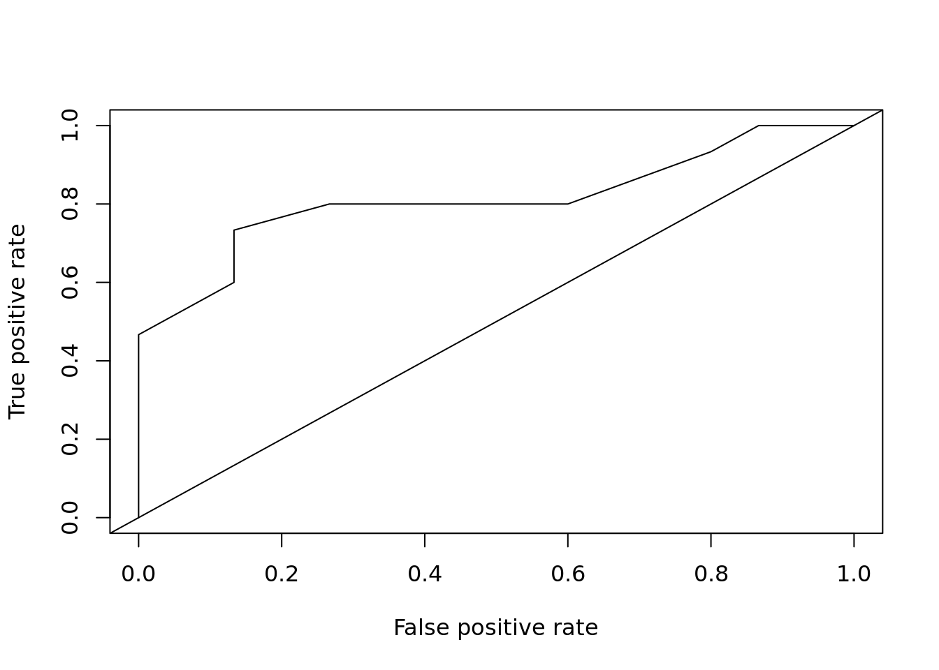
## [1] 0.8111111rf <- randomForest::randomForest(Species ~ ., data = train)
plot_roc_get_auc(
pred = predict(rf, test[, 1:4], type = "prob")[,'versicolor'],
test_labels = as.integer(test[["Species"]]) - 1)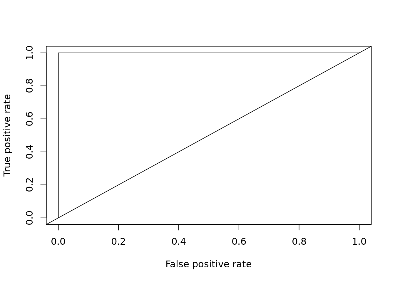
## [1] 1cross-validation
TODO
ROC - TPR vs FPR, where
TPR - True Positive Rate TP - True Positive FP - False Positive
parameter search
https://scikit-learn.org/stable/modules/grid_search.html#tuning-the-hyper-parameters-of-an-estimator
TODO: https://rviews.rstudio.com/2019/03/01/some-r-packages-for-roc-curves/
TODO: https://www.saedsayad.com/model_evaluation_c.htm