1. What is tidyverse and why would you use it?
tidyverse is a collection of R packages that make working on data a much nicer experience comparing to base R;
it consists of tidyr, dplyr, ggplot2, tibble and a few more.
To be honest, I prefer data.table to tidyverse, as it resembles basic R data.frames, is faster, more concise and, IMHO, more SQL-ish. But it takes longer to master and may be more difficult to understand, even your own code after some time. So, there is no obvious choice between data.table and dplyr.
2. A few “Hello World” examples
readr
Or how we read and write data in tidyverse.
Nobody uses basic R functions to read tabular data anymore. data.table::fread() and readr::read_csv() are smarter and faster.
Let’s create a sample dataset:
sample_data <- data.frame(
  col_a = letters[1:5],
  col_b = sample(1:100, 5)
)

class(sample_data)
## [1] "data.frame"Then let’s write it and read back to R:
readr::write_csv(x = sample_data, path = 'sample_data.csv')## Warning: The `path` argument of `write_csv()` is deprecated as of readr 1.4.0.
## Please use the `file` argument instead.
## This warning is displayed once every 8 hours.
## Call `lifecycle::last_warnings()` to see where this warning was generated.data_t <- readr::read_csv(file = 'sample_data.csv')## Rows: 5 Columns: 2## -- Column specification --------------------------------------------------------
## Delimiter: ","
## chr (1): col_a
## dbl (1): col_b##
## i Use `spec()` to retrieve the full column specification for this data.
## i Specify the column types or set `show_col_types = FALSE` to quiet this message.As you can see, readr was happy to inform us that it imported column col_a as characters and column col_b as integers, which is exactly what we wanted. You can customise this behaviour. How to do it? readr has an extensive documentation ;).
The data we read is an object of class “tibble”, which has a nice printing method.
class(data_t)## [1] "spec_tbl_df" "tbl_df" "tbl" "data.frame"print(data_t)## # A tibble: 5 x 2
## col_a col_b
## <chr> <dbl>
## 1 a 28
## 2 b 25
## 3 c 32
## 4 d 53
## 5 e 71Tibbles do not differ much from data.frames, except (according to the documentation, i.e. ?tibble::tibble):
‘tibble()’ is a trimmed down version of ‘data.frame()’ that:
• Never coerces inputs (i.e. strings stay as strings!).
• Never adds ‘row.names’.
• Never munges column names.
• Only recycles length 1 inputs.
• Evaluates its arguments lazily and in order.
• Adds ‘tbl_df’ class to output.
• Automatically adds column names.
‘data_frame()’ is an alias to ‘tibble()’.
Btw, to create a tibble by hand, you use:
tibble::data_frame(a = 1:5, b = letters[1:5])## Warning: `data_frame()` was deprecated in tibble 1.1.0.
## Please use `tibble()` instead.
## This warning is displayed once every 8 hours.
## Call `lifecycle::last_warnings()` to see where this warning was generated.## # A tibble: 5 x 2
## a b
## <int> <chr>
## 1 1 a
## 2 2 b
## 3 3 c
## 4 4 d
## 5 5 eSo it’s exactly the same as creating a usual data.frame.
dplyr
Or smart SQL (DDL + DML) in R.
Let’s have a look at the most common expressions:
library(dplyr)##
## Attaching package: 'dplyr'## The following objects are masked from 'package:stats':
##
## filter, lag## The following objects are masked from 'package:base':
##
## intersect, setdiff, setequal, unionAs you can see, if you use function filter(), the one from dplyr package will be run.
mtcars %>%
    select(mpg, cyl, disp) %>%
    filter(cyl == 8) %>%
    arrange(-disp) %>%
    mutate(col_a = cyl * 2, col_b = "hi") %>%
    head()
## mpg cyl disp col_a col_b
## Cadillac Fleetwood 10.4 8 472 16 hi
## Lincoln Continental 10.4 8 460 16 hi
## Chrysler Imperial 14.7 8 440 16 hi
## Pontiac Firebird 19.2 8 400 16 hi
## Hornet Sportabout 18.7 8 360 16 hi
## Duster 360 14.3 8 360 16 hiWhat happened here:
we used one of basic R datasets: mtcars;
we piped it with
%>%to the next function (piping, or pipelines, is one of the oldest Unix concepts, dating back to 1970s);we used a
selectto select columns we were interested in, just like in SQL;we used a
filterfunction just as SQL’swhereclause;we ordered the dataset with
arrange;we added two new columns with
mutate;we used a
head()function to print only a few first rows of our dataframe.
An example of grouping:
mtcars %>%
    group_by(cyl) %>%
    summarise(count = n(), mean_hp = mean(hp))
## # A tibble: 3 x 3
## cyl count mean_hp
## <dbl> <int> <dbl>
## 1 4 11 82.6
## 2 6 7 122.
## 3 8 14 209.What happened here:
we aggregated our data with
group_byin the same way as we do in SQL;we wrote the aggregation functions:
n()stands for number of objects orcountin SQL andmean()is an example of an aggreagtion function (sum,sd,median, …)
Another example of grouping, with count (count is exactly the same as group_by() %>% summarise(n = n()), but shorter):
mtcars %>%
    count(cyl)
## cyl n
## 1 4 11
## 2 6 7
## 3 8 14ggplot2
I prepared a separate tutorial for ggplot2.
3. Curiosities
- you can pipe your data directly to ggplot2
library(dplyr)
library(ggplot2)

mtcars %>%
    filter(gear >= 4) %>%
    ggplot(mapping = aes(x = mpg, y = cyl)) +
    geom_point()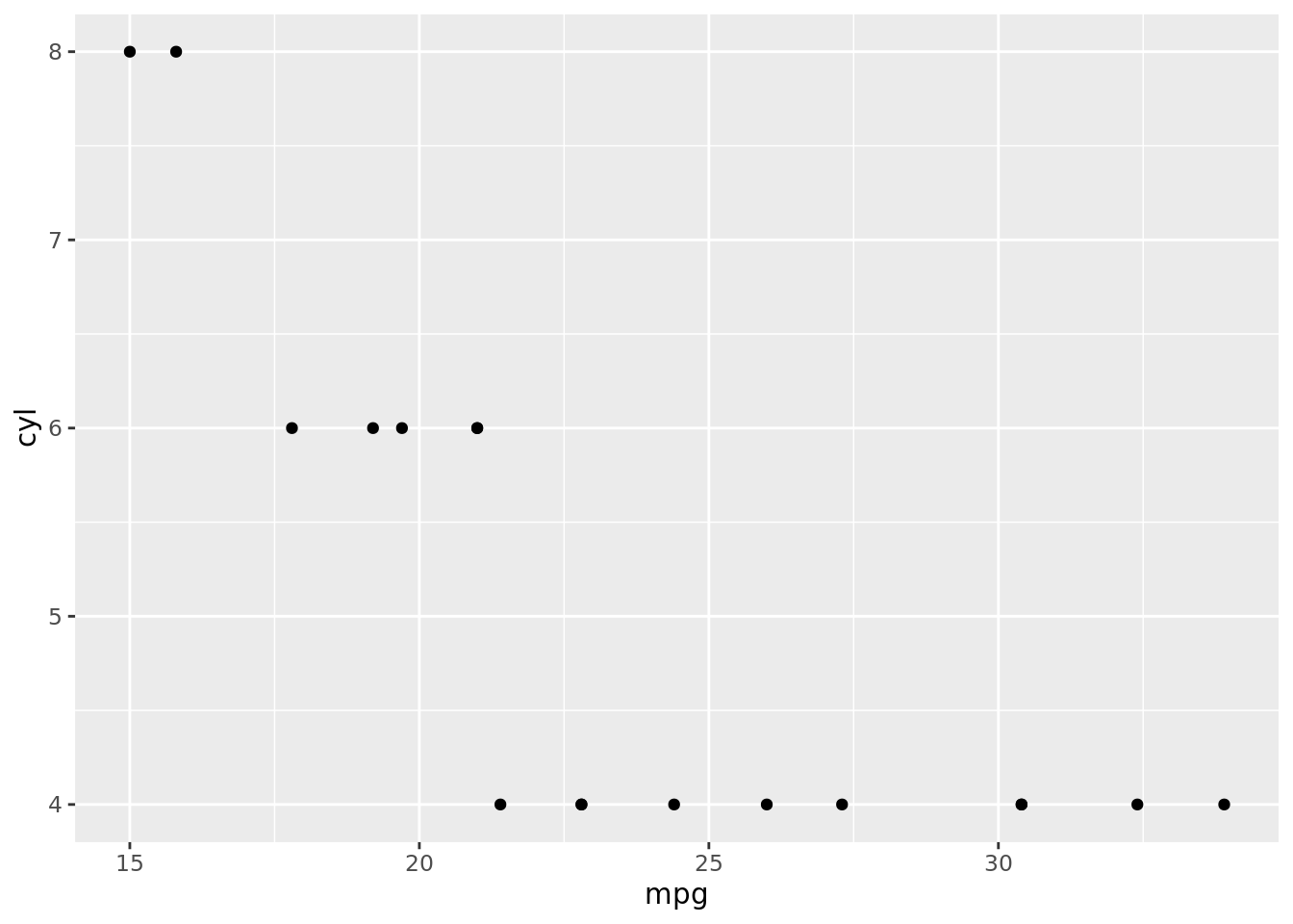
But remember that in ggplot2 we use + for piping, not %>%. There is an easy way to never forget about it: use data.table instead of dplyr ;).
- you can use
%>%operators on any class of data you like, e.g.:
data.table::as.data.table(mtcars) %>%
    filter(mpg > 21) %>%
    select(mpg, cyl) %>%
    head()
## mpg cyl
## 1: 22.8 4
## 2: 21.4 6
## 3: 24.4 4
## 4: 22.8 4
## 5: 32.4 4
## 6: 30.4 44. Subjects still to cover
dplyr: joins, slice, spread, separate/unite (TODO) (spread is dcast)
table of contents