1. What is nls and why would you use it?

• nls, or nonlinear least squares is a statistical method used to describe a process as a nonlinear function of deterministic variables and a random variable;

• you may think of it as an older and stronger brother of linear regression - more robust, powerful, smarter and difficult to understand ;)

2. A “Hello World” example

Let’s assume we want to model US population as a function of year.

USPop <- data.frame(
  year = seq(from = 1790, to = 2000, by = 10),
  population = c(3.929, 5.308, 7.240, 9.638, 12.861, 17.063, 23.192, 31.443, 
                 38.558, 50.189, 62.980, 76.212, 92.228, 106.022, 123.203, 
                 132.165, 151.326, 179.323, 203.302, 226.542, 248.710, 281.422)
)

plot(population ~ year, data = USPop, 
     main = "US population over the last 200 years or so")
abline(lm(population ~ year, data = USPop), col = "red", lwd = 2)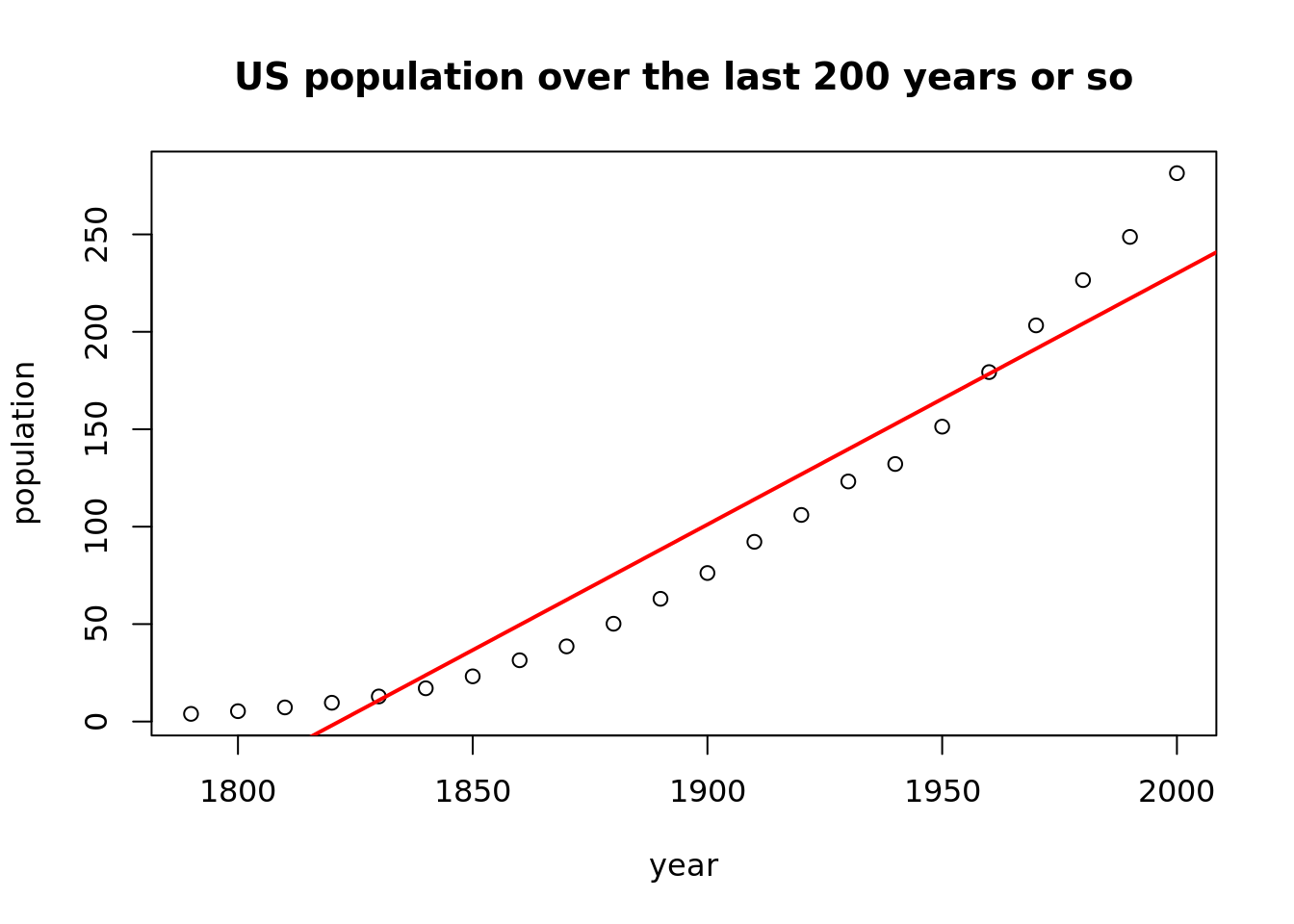

USPop dataset used to be available in car package, curiously it isn’t anymore.

Yeah, I love these statistical, ascetic plots. The black line is a line proposed by linear regression and as we can see, it does not really fit the data. We can observe a rising trend, but it definitely is not linear. Modeling this process as a nonlinear function of year seems to be a reasonable approach.

But what kind of nonlinear function should we use? One of the most popular nonlinear functions is a logistic function. In this case we will use it’s more general form, in which the maximum value of the function is not 1, but \(\theta_1\):

\[ f(\textrm{year}) = \frac{\theta_1}{1 + e^{-(\theta_2 + \theta_3 * \textrm{year})}} \]

Before we’ll move to the estimation of the parameters, let’s calculate starting values for minimisation (least squares) algorithm. Natural candidates would be coefficients of linear regression, where our dependent variable is linearised with a logit() function. Note that in this linearised model we will not estimate the Intercept, as we scale the dependent variable by diving all the values by a little more than it’s maximum, so that \(\textrm{population}\in(0,1)\). Our estimation of the Intercept is this maximum value that we divided by.

t1 <- max(USPop$population) * 1.05
model_start <- lm(car::logit(population / t1) ~ year, USPop)
starts <- c(t1, model_start$coefficients)
names(starts) <- c("theta1", "theta2", "theta3")
print(starts)

##       theta1       theta2       theta3 
## 295.49310000 -57.46319522   0.02968818

Having the starting values for parameters ready, we can move on to using the nls function, which will calculate the final parameters.

form <- population ~ theta1  / (1 + exp(-(theta2 + theta3 * year)))
model <- nls(formula = form, data = USPop, start = starts)
print(model)

## Nonlinear regression model
##   model: population ~ theta1/(1 + exp(-(theta2 + theta3 * year)))
##    data: USPop
##    theta1    theta2    theta3 
## 440.83108 -42.70710   0.02161 
##  residual sum-of-squares: 457.8
## 
## Number of iterations to convergence: 7 
## Achieved convergence tolerance: 7.271e-06

As we can see, the estimated parameters values do not differ much from starting values. Which was rather expected.

The plot below presents a much better fit of a model with logistic function, comparing to linear regression.

plot(population ~ year, data = USPop, 
     main = "US population over the last 200 years or so")
USPop$fitted_values <- fitted(model)
lines(fitted_values ~ year, data = USPop, col = "blue", lwd = 2)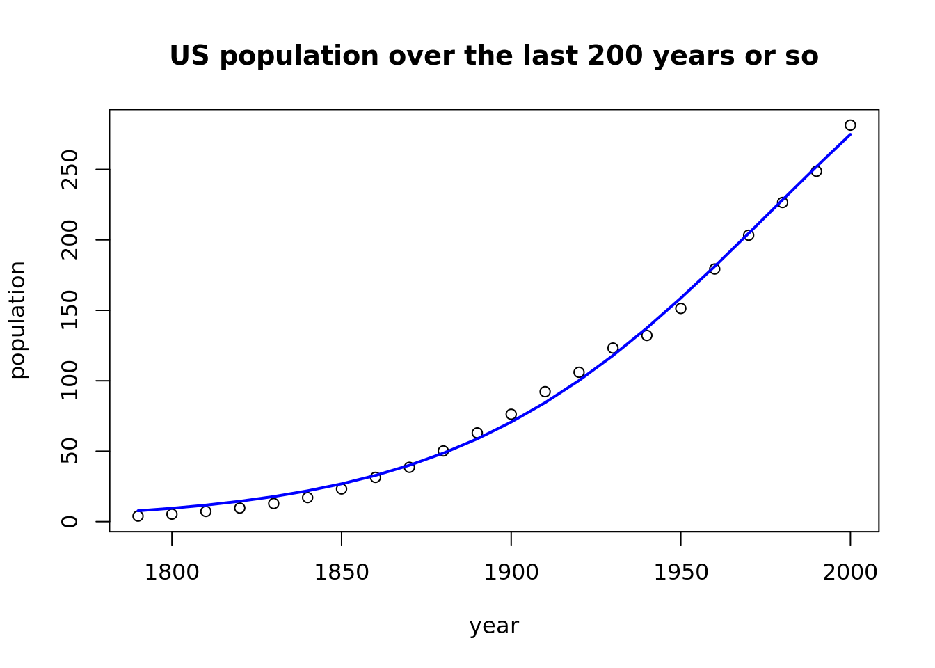

3. Afterthoughts

• using nls() in fact does not differ much from using standard ls();

• to solve nonlinear problems with nls, we can use any function, not only logistic regerssion.