Why would you use delta table?
When you work on huge amounts of data, you probably use spark as querying engine and store data either in spark on in a cloud storage (S3 / Google Cloud Storage / Azure Storage), which together nring architecure called data lake.
Vast amounts of data are still in tabular format, so you may feel tempted to store them in a data warehouse, because of its nice features, like ACID and locking. On the other hand, data warehouses do not scale (almost) indefinitely, like data lakes.
Delta lake, which is a group of delta tables is an implementation of a data lakehouse, which combines advantages of data lakes and warehouses:
-
(almost) indefinite scaling
-
ACID and locking (gaining functionality equivalent to data warehouse requires additional tools, but by default we get some sort of locking)
-
as a bonus we get data versioning, which is called
time travel, and uses data partitioning in a clever way
Currently delta tables are heavily used by databricks, which is a PaaS solution to run spark clusters on data stored in cloud (AWS/GCP/Azure).
Example project
Introduction
We want to find out if SUVs are getting more and more popular in the US.
To do that, we download data on cars manufacturers: to be more specific, what car body types were available on the American market from 2003 to 2023, based on the data from https://github.com/abhionlyone/us-car-models-data. The data is published in the following way:
-
in CSV format,
-
one CSV file per year, which contains car models sold on American market with the information on body style (e.g. SUV, sedan, wagon, convertible, etc).
Architecture
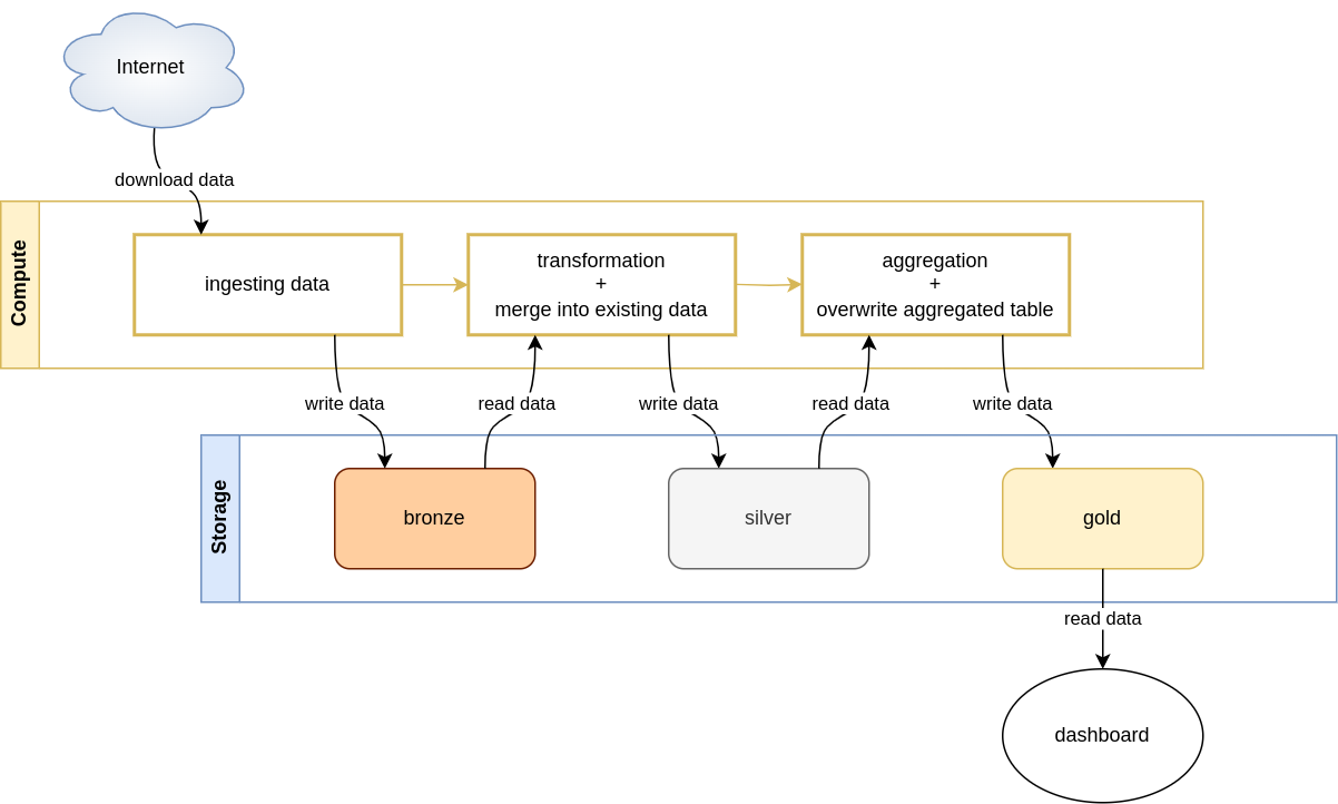
The architecture can be divided into 2 components:
-
Compute, where 3 tasks reside. In production setting they might be orchestrated by a pipeline orchestrator like airflow (I also wrote about using airflow with BigQuery [here]https://greysweater42.github.io/airflow_bigquery/). For this particular project we want to use
delta tables, which are in general data formats that can be accessed by multiple processing engines, like spark. The popular engines are currently spark and custom engine written in rust, which allows only read and write queries, without any data manipulation. Any other data manipulation engine can be used, so we will used pandas (polars is also a popular choice). In this blog post I will show examples of both spark and delta-rs + pandas. -
Storage, where the medallion architecture is used. In short, it consists of 3 layers, called: bronze, silver, and gold, and each of these contains cleaner data. Bronze is for raw data (no delta tables), silver for cleaned data (delta tables) and gold for aggregated clean data (delta tables). You may find more information about this architecture in Delta lake: Up and Running book.
Implementation
Prerequsites
We will need a couple of python packages:
requirements.txt
delta-spark==3.1.0
deltalake==0.17.4
pyspark==3.5.1
pandas==2.2.2
You might want to install other versions of these packages. In worst case scenario, you will have to debug the code below by yourself.
You might rather use spark docker container instead of installing it in virtualenv. Virtualenv worked well for me.
Project structure
Our project consists of a couple of components, in particular we might divide them into: spark and pandas, and separate tasks. I recommed the following project structure:
.
├── config.py
├── main.py
└── src
    ├── aggregate_pandas.py
    ├── aggregate_spark.py
    ├── extract.py
    ├── setup_spark.py
    ├── transform_pandas.py
    └── transform_spark.py
Now lets have a look at each of the files of the project.
config
config.py
from pathlib import Path
from dataclasses import dataclass
from collections import OrderedDict

from pyspark.sql import types
import numpy as np


DATA_PATH = Path("data")


@dataclass
class DATA_PATHS:
    bronze = DATA_PATH / "bronze"
    silver = DATA_PATH / "silver"
    gold = DATA_PATH / "gold"


DATA_PATHS.bronze.mkdir(exist_ok=True, parents=True)
DATA_PATHS.silver.mkdir(exist_ok=True, parents=True)
DATA_PATHS.gold.mkdir(exist_ok=True, parents=True)

URL = (
    "https://raw.githubusercontent.com/abhionlyone/us-car-models-data/master/{year}.csv"
)
# we process 21 years: from 2003 to 2023
YEARS = range(2003, 2024)

# in silver layer we merge new batch (new year) into existing data on condition
# to avoid overwriting existing rows
MERGE_CONDITION = " and ".join(
    [
        "cars.year = new_data.year",
        "cars.make = new_data.make",
        "cars.model = new_data.model",
        "cars.body_style = new_data.body_style",
    ]
)

# we store schema of the tables here in an attempt to separate DDL from DML
SCHEMA_SPARK = types.StructType(
    [
        # we use short type for compatibility with pandas: pandas uses 64bit int
        # by default, spark uses 32. if we need to specify them manually, let's
        # choose ShortType (8-bit), which is enough for storing year
        types.StructField("year", types.ShortType(), True),
        types.StructField("make", types.StringType(), True),
        types.StructField("model", types.StringType(), True),
        # unfortunately spark doesn't allow reading arrays from csvs directly
        types.StructField("body_styles", types.StringType(), True),
    ]
)

# we use short type for compatibility with spark: pandas uses 64-bit int by
# default, while spark uses 32 bit. we need to override the defaults, so we use
# 8-bit short (also known as int16), because we save a little bit of space.
# OrderedDict instead of dict, because we want to keep the order of the columns
# for nicer default
SCHEMA_PANDAS = OrderedDict(year=np.short, make=str, model=str, body_styles=str)
main
from datetime import datetime

import config

from src.extract import extract
from src.transform_pandas import transform
from src.aggregate_pandas import aggregate

# from src.setup_spark import setup_dev_spark_session
# from src.transform_spark import transform
# from src.aggregate_spark import aggregate

if __name__ == '__main__':
    for year in config.YEARS:
        t0 = datetime.now()
        print(year)
        raw_data_path = extract(year=year)
        transformed_data_path = transform(raw_data_path=raw_data_path)
        aggregate(transformed_data_path=transformed_data_path)
        # spark = setup_dev_spark_session()
        # transformed_data_path = transform(spark=spark, raw_data_path=raw_data_path)
        # aggregate(spark=spark, transformed_data_path=transformed_data_path)
        print(datetime.now() - t0)
Yes, I used print instead of logging, because this is not production code.
This script iterates over 21 years and for each of the years runs the pipeline as is depicted in the architecture diagram: downloads one year of data, saves it into bronze layer, then cleans the data and finally aggregates it to save the result to the gold layer. Dashboard is not implemented.
Some sections are commented out. The uncommented code runs the pipeline using delta-rs and pandas. The commented out sections use spark. If you uncomment them and comment the other functions from src, processing will be run using spark. You will notice that running the processing in spark is significantly slower that delta-rs + pandas, because the dataset is very small (normally for such a small dataset we would not even consider using spark, but this is just an example). For bigger datasets (terabytes of data) we would not manage to run such a processing with pandas at all. You might also run transforming with pandas and aggregating with spark or transforming with spark and aggregating with pandas, if you want. They both use the same delta table format.
In the code above you can see that the functions run in the for loop correspond to tasks in the architecture diagram: extract, transform, and aggregate. transform also performs merging and aggregate also performs overwriting data in the gold layer.
extract
This is the first part of the pipeline: downloads data from the internet.
src/extract.py
from pathlib import Path

import pandas as pd

import config


def extract(year: int) -> Path:
    """reads raw cars csv file for a given year from the internet and saves it
    to data path to the bronze layer. If the file already exists there,
    downloading is skipped"""
    path = (config.DATA_PATHS.bronze / "cars" / str(year)).with_suffix(".csv")
    path.parent.mkdir(parents=True, exist_ok=True)

    if not path.exists():
        url_year = config.URL.format(year=year)
        df = pd.read_csv(url_year)
        df.to_csv(path, index=False)
    return path
setup spark
As we’re moving to the second task of the pipeline, which is cleaning (transforming) the data, we need an important prerequisite to run the processing using spark: a spark session. For this blog post we setup a dev spark cluster with one worker node (it’s more than enough anyway). You will find more information about local setup on delta lake’s getting started page.
src/setup_spark.py
from pyspark.sql import session
from delta import configure_spark_with_delta_pip


def setup_dev_spark_session() -> session.SparkSession:
    builder = (
        session.SparkSession.builder.appName("MyApp")
        .config("spark.sql.extensions", "io.delta.sql.DeltaSparkSessionExtension")
        .config(
            "spark.sql.catalog.spark_catalog",
            "org.apache.spark.sql.delta.catalog.DeltaCatalog",
        )
    )

    # this environment should be used only for testing
    # more info here https://delta.io/learn/getting-started/
    spark = configure_spark_with_delta_pip(builder).getOrCreate()
    return spark
transform with pandas
src/transform_pandas.py
import json
from pathlib import Path

import deltalake as dl
import pandas as pd

import config


def _explode_cars_on_body_style(df: pd.DataFrame) -> pd.DataFrame:
    """`body_styles` column is an array, which csv keeps as a string.
    This function converts it into actual array and explodes it.
    """
    df["body_styles"] = df["body_styles"].apply(lambda x: json.loads(x))
    return df.explode("body_styles").rename({"body_styles": "body_style"}, axis=1)


def transform(raw_data_path: Path) -> Path:
    """cleans raw data and saves it to silver layer as a delta table"""
    clean_data_path = config.DATA_PATHS.silver / "cars"

    # we could probably read the `body_styles` column as a pyarrow array/list type
    new_batch_raw = pd.read_csv(
        raw_data_path, usecols=config.SCHEMA_PANDAS.keys(), dtype=config.SCHEMA_PANDAS
    )
    new_batch_clean = _explode_cars_on_body_style(df=new_batch_raw)

    if not clean_data_path.exists():
        dl.write_deltalake(
            clean_data_path, new_batch_clean, partition_by=["year", "body_style"]
        )
    else:
        clean_data = dl.DeltaTable(clean_data_path)
        (
            clean_data.merge(
                source=new_batch_clean,
                predicate=config.MERGE_CONDITION,
                source_alias="new_data",
                target_alias="cars",
            )
            .when_not_matched_insert_all()
            .execute()
        )

    return clean_data_path
Our body_styles column comes in an interesting format: it is a json array. COnsidering that the data is stored in a CSV file, we need to read it as string and then convert to json array. And then we explode the data on this column to finally get rid of this array, which would make further processing difficult.
The transform function has an if statement inside. We process the data year by year and we always merge the new batch to an already existing delta table. But what if it is the first batch ever? Then we create a new delta table.
The data is partitioned by two columns: year and body_style. Year is convenient, because we receive the data per year, so a new batch of the data does not modify already existing partitions. In other words, appending a new year of data is very cheap and efficient. Partitioning on body_style will make filtering on this column faster. (Obviously for such a small dataset with ~500 rows per year we actually de-optimize the performance by introducing way too many files/partitions, which is an overhead for spark and delta).
transform with spark
src/transform_spark.py
from pathlib import Path

from delta.tables import DeltaTable
from pyspark.sql import functions as F, dataframe, session, types

import config


def _explode_cars_on_body_style(
    df: dataframe.DataFrame,
) -> dataframe.DataFrame:
    """`body_styles` column is an array, which csv keeps as a string.
    This function converts it into actual array and explodes it.
    """
    df = df.withColumn(
        "body_styles",
        F.from_json(df["body_styles"], types.ArrayType(types.StringType())),
    )
    return df.select(
        "year", "make", "model", F.explode("body_styles").alias("body_style")
    )


def transform(spark: session.SparkSession, raw_data_path: Path) -> Path:
    """cleans raw data and saves it to silver layer as a delta table"""
    clean_data_path = config.DATA_PATHS.silver / "cars"

    new_batch_raw = spark.read.csv(
        str(raw_data_path), header=True, schema=config.SCHEMA_SPARK, escape='"'
    )
    new_batch_clean = _explode_cars_on_body_style(df=new_batch_raw)

    if not clean_data_path.exists():
        new_batch_clean.write.format("delta").save(
            str(clean_data_path), partitionBy=["year", "body_style"]
        )
    else:
        clean_data = DeltaTable.forPath(spark, str(clean_data_path))
        clean_data.alias("cars").merge(
            new_batch_clean.alias("new_data"), config.MERGE_CONDITION
        ).whenNotMatchedInsertAll().execute()

    return clean_data_path
This code is (surprisingly) similar to transform_pandas.py.
aggregate in pandas
src/aggregate_pandas.py
from pathlib import Path

import deltalake as dl

import config


def aggregate(transformed_data_path: Path) -> Path:
    """aggregates transformed cars data by year and body style and writes the
    result to the gold layer"""
    agg_data_path = config.DATA_PATHS.gold / "cars"

    df = dl.DeltaTable(transformed_data_path).to_pandas()
    # I could have written the following lines as one line, but this syntax makes
    # debugging easier
    df["is_SUV"] = df["body_style"] == "SUV"
    df = df.groupby(["year", "is_SUV"]).count().reset_index()
    df = df.pivot(columns="is_SUV", index="year", values="model")
    df = df.rename({False: "not_SUV", True: "SUV"}, axis=1)
    df["all"] = df["SUV"] + df["not_SUV"]
    df["SUV_market_share"] = round(df["SUV"] / df["all"], 2)

    dl.write_deltalake(agg_data_path, df, mode="overwrite")
    return agg_data_path
aggregate in spark
src/aggregate_spark.py
from pathlib import Path

from pyspark.sql import session, functions as F

import config


def aggregate(spark: session.SparkSession, transformed_data_path: Path) -> Path:
    """aggregates transformed cars data by year and body style and writes the
    result to the gold layer"""
    agg_data_path = config.DATA_PATHS.gold / "cars"

    df = spark.read.format("delta").load(str(transformed_data_path))
    # I could have written the following lines as one line, but this syntax makes
    # debugging easier
    df = df.withColumn("is_SUV", F.col("body_style") == "SUV")
    df = df.groupby(["year", "is_SUV"]).count()
    df = df.groupBy("year").pivot("is_SUV").sum("count")
    df = df.withColumnRenamed("false", "not_SUV").withColumnRenamed("true", "SUV")
    df = df.withColumn("all", F.col("SUV") + F.col("not_SUV"))
    df = df.withColumn("SUV_market_share", F.round(F.col("SUV") / F.col("all"), 2))

    df.write.format("delta").mode("overwrite").save(str(agg_data_path))
    return agg_data_path
Note on time travel
Time travel is implemented in a very interesting way: whenver we make a change to the delta table (whether it’s an insert, update, or delete), only those partitions where this change happened are modified. What does ‘modify’ mean here? It’s not overwriting, but creating a new partition and storing the information on which partitions belong to this particular of the version of the table in a separate file, called transaction log (or delta log). Effectively, a delta table format consists of two types of files: a json file to store the information on history, versions, and partitions of the table, and the partitions themselves stored as parquet files.
When the processing is done, you might want to review the historical versions of the gold table with the following commands:
for pandas
import deltalake as dl
import pandas as pd


path = "data/gold/cars"

# history as json
print(dl.DeltaTable(path).history())
# history as table
print(pd.DataFrame(dl.DeltaTable(path).history()))

# prints a df with one record: for 2003
print(DeltaTable(path, version=0).to_pandas())
# prints a df with 2 records: dor 2003 and 2004
print(DeltaTable(path, version=1).to_pandas())

dt = DeltaTable(path)
dt.load_as_version(1)
# prints a df with two records: for 2003 and 2004
print(dt.to_pandas())
for spark
from src.setup_spark import setup_dev_spark_session
from delta.tables import DeltaTable


path = "data/gold/cars"

spark = setup_dev_spark_session()

# read version 0 (the oldest) of the gold table
df = spark.read.format("delta").option("versionAsOf", 0).load(path)
print(df.show())

# version history
deltaTable = DeltaTable.forPath(spark, path)
print(deltaTable.history().show())
Other remarks
-
Since the data is stored in parquet files,
delta-rsimplementation sometimes uses pyarrow objects (e.g. schema) for more low-level uses -
When we performed aggregation in the last step, we reprocessed all the previous years, while we could process only the new year and append it into the gold layer table. For a big dataset the performance would be significantly better.