1. Why yet another article about Bayes’ theorem and bayesian inference?

There seem to be enough of them on the net.

From my perspective the articles available on the internet (by internet I mean medium or towardsdatascience) are:

• written from the probabilistic/mathematical point of view, which has little in common with statistical inference, which is the practical use of Bayes’ theorem (italics is a small wink at mathematicians, whose work is usually theoretical) and concentrate on the intution, which fits mathematical perspective, but not statistical

• inversly-chronological. They start reasoning from the equation, which IMHO is the inverse of reasoning; the equation describes the thought, the idea or the intuition of any phenomenom, so the equation is a result of an idea that we are trying to grasp. We should start with the idea, not the equation.

• do not relate to, well, pretty much anything. People who are trying to understand Bayes’ theorem and bayesian inference usually have statistical or computer science/machine learning background, and Bayes’ theorem resembles quite a lot of concepts from these fields. In most articles it is presented as something utterly different to, well, anything.

• do not match bayesian inference with Bayes’ theorem, probably because of using different abstractions to visualize how these two equations work. I alwayys felt like using Bayes’ theorem for bayesian inference is some sort of trick (But if we do that clever interpretation, where A is a parameter and B is data, then…). Relying on a clever trick is faster, but risky: deep understading is a much safer approach.

I will try to adress all of the flaws above.

2. Gaining intuition

circles and areas

Probably the most common way of presenting intuition to anything is by showing a picture. Bayes’ theorem can be shown on a graph as well: a graph presenting e.g. two slightly overlapping circles:

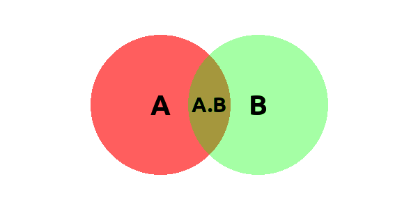
We can see two areas: A and B, which overlap and have a common area: A.B. We may amuse ourselves with a short riddle:

Knowing I am in B, what is the probability that I am in A?

May sound simple enough and we denote it as conditional probability:

$$ P(A|B) = \frac{P(A\cap B)}{P(B)} $$

which means we clearly are in an area denoted as A.B ($A \cap B$, in other words), but we know that we are surely, 100%, in B, so the probability of being in B is one. Hence we adjust our perspective to be surely in B by dividing by P(B).

Personally I find it easier to think of areas instead of probabilities. If area of A.B is 2, and area of B is 10, then the chance of being in A.B given B is 0.2.

But conditional probability is not Bayes’ theorem yet. We can rewrite the nominator using conditional probability:

$$ P(A|B) = \frac{P(B|A) \cdot P(B)}{P(B)} $$

which is a little more difficult to understand graphically, but still possible. Now the nominator is a funny expression showing that the common area can be denoted in terms of conditional probability. The best way to see it is making a few drawing by yourself (it took me maybe 3 hours until I actually felt it). One transformation turned out to particurarily useful, the moment I saw it in terms of circles in my head:

$$ P(A\cap B) = P(A|B) \cdot P(B) = P(B|A) \cdot P(B) $$

The intersection can be described in two symmetrical ways, by referring both to A and B and their conditional probabilities.

Yet still there is one more sophistication: we can rewrite the probability of B in the context of conditional probabilities of A:

$$ P(B) = P(B|A) \cdot P(A) + P(B|\neg A) \cdot P(\neg A) = \Sigma_{A^*} P(B|A^*) \cdot P(A^*) $$ where $$ A^* = {A, \neg A } $$

which for the moment seem to serve to purpose. It seems fairly obvious that P(B) is equal to the intersection of B and A plus the intersection of B and everything that is not A. In the case of circles, it is useless (at least for me), but for bayesian inference, it is crucial.

Unfortunately, this “circle/area” intuition cannot be used to understand bayesian inference whatsoever. Imagine the following example:

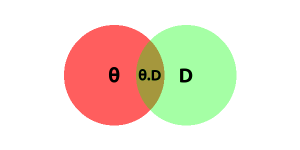
I don’t think is it possible to interpret the intersection of parameters and data as the common area of these two sets. So other visualizations must be used to understand it.

contingency table

is often used in statistics to analyze distributions of two random variables, e.g. $X$ and $Y$. It is useful, because one can pretty easily see if the variables are correlated/dependent (condition for independence: $P(A \cap B) = P(A) \cdot P(B)$ for every possible values of $A$ and $B$).

In machine learning a contingency table is usually used for model validation in a form of confusion matrix, with its derivative metrics: precision/recall, sensitivity/specificity etc. The elements of a confusion matrix can also be interpreted as I and II type errors (respectively: FP and FN).

As you can see, contingency table can express basic concepts of machine learning (confusion matrix), statistics (hypothesis testing) and bayesian inference (marginal distributions), which helps building your knowledge on concepts you already know.

There are two popular versions of contingency table: with probabilities and with counts. The only difference is that the latter is multiplied by n (number of observations), beside the obvious differences in interpretation.

A contingency table in its basic form, for random variables looks like this:

$$ \begin{array}{cc|cc|c} & & \pmb{X} & \\ & & 1 & 0 & \Sigma \\ \hline \pmb{Y} & 1 & 0.1 & 0.3 & 0.4 \\ & 0 & 0.4 & 0.2 & 0.6 \\ \hline & \Sigma & 0.5 & 0.5 & 1 \\ \end{array} $$

in case of probabilities. Confusion matrices have integers, not fractions. In the example above I used two random variables: $X$ and $Y$, but they can be called anyhow, e.g. $\theta$ and $D$:

$$ \begin{array}{cc|cc|c} & & \pmb{\theta} & \\ & & 1 & 0 & \Sigma \\ \hline \pmb{D} & 1 & 0.1 & 0.3 & 0.4 \\ & 0 & 0.4 & 0.2 & 0.6 \\ \hline & \Sigma & 0.5 & 0.5 & 1 \\ \end{array} $$

which will give us a feel of bayesian inference. Let’s see how we can derive the table above:

$$ \begin{array}{cc|cc|c} & & \pmb{\theta} & \\ & & \theta = 1 & \theta = 0 & \Sigma \\ \hline \pmb{D} & D = 1 & P(\theta = 1 \cap D = 1) & P(\theta = 0 \cap D = 1) & P(\theta = 1 \cap D = 1) + P(\theta = 0 \cap D = 1) \\ & D = 0 & P(\theta = 1 \cap D = 0) & P(\theta = 1 \cap D = 0) & P(\theta = 1 \cap D = 0) + P(\theta = 0 \cap D = 0) \\ \hline & \Sigma & P(\theta = 1 \cap D = 1) + & P(\theta = 0 \cap D = 1) + & 1 \\ & & + P(\theta = 1 \cap D = 0) & + P(\theta = 0 \cap D = 0) & \\ \end{array} $$

and let’s see if we can derive any of the rows (we could do the same for columns) as we are well equipped with our brand new knowledge of Bayes’ theorem.

$$ \begin{array}{cc|cc|c} & & \pmb{\theta} & \\ & & \theta = 1 & \theta = 0 & \Sigma \\ \hline \pmb{D} & D = 1 & P(D=1|\theta=0)\cdot P(\theta=0) & P(D=1|\theta=1)\cdot P(\theta=1) & \Sigma_{\theta^*}P(D=1|\theta=\theta^*) \cdot P(\theta=\theta^*) \\ \end{array} $$

we could obviously substitute probability intersections with their symmetrical conditionals, because

$$ P(\theta \cap D) = P(\theta|D) \cdot P(D) = P(D|\theta) \cdot P(\theta) $$

but in the rightmost column where we have the sum, it has a slightly nicer interpretation: $D$ is equal to 1, e.g. is constant in the whole row, and the sum itself is called marginal likelihood and in bayesian statistics is often called shortly evidence and denoted as $P(D)$. As we can see, it must be equal to $P(D)$, as we sum over all the possible values of $\theta$, so it’s the probability of D regardless of the value of $\theta$.

What we see in the table above is a specific case for variables which take values of 0 and 1. Sometimes we want to abstract from specific values of $\theta$ and $D$, as there may be many of them, up to infinity, even. Then we can rewrite the table above as the following:

$$ \begin{array}{cc|ccc|c} & & & \pmb{\theta} & & \\ & & … & \text{some}~\theta & … & \Sigma \\ \hline & … & … & … & …\\ \pmb{D} & \text{some}~D & … & P(D|\theta)\cdot P(\theta) & …& \Sigma_{\theta^*} P(D|\theta^*) \cdot P(\theta^*) \\ & … & … & … & …\\ \hline & \Sigma & … & \Sigma_{D^*}P(\theta|D^*) \cdot P(D^*) & …\\ \end{array} $$

from which we can deduce a value

$$ \frac{P(D|\theta)\cdot P(\theta)}{\Sigma_{\theta^*} P(D|\theta^*) \cdot P(\theta^*)} $$

which is obviously equal to $P(\theta|D)$, as Bayes’ theorem states. Just as in the basic example with $X$ and $Y$ random variables, conditional probability of $\theta$ given $D$ is their intersection divided by the whole $D$.

Now imagine that $\theta$ and $D$ have continuous distributions. In this case in order to calculate the denominator of the equation above we would have to add up infinitely many numbers. In mathematics there is even a special notation (abstraction) for that: the integral. Hence we can rewrite the Bayes’ theorem for continuous variables:

$$ P(\theta|D) = \frac{P(D|\theta)\cdot P(\theta)}{\int d \theta^* ~ P(D|\theta^*) \cdot P(\theta^*)} $$

See? We’ve just exchanged $\Sigma_{\theta^*}$ with $\int d \theta^*$. (Computationally it is slightly more complicated than just replcaing a symbol with one eanother, since many posterior distributions are impossible to solve analytically, and numeric metods must be used, like MCMC).

3. References

The best book on Bayes’ theorem and bayesian inferece is Doing Bayesian Analysis by John K. Kruschke and many examples I gave in this blogpost were my own interpretations of some chapters of this book.

4. TODO

• TODO connection between circles and contingency table - contingency table is a generalized picture of circles

• TODO precision and recall, sensitivity and specificity - specificity/sensitivity - rationality, thinking fast and slow: example with drug specificity/sensitivity and precision

• TODO type I and type II errors (CI and power) - Mixing up bayesian and frequentist inference may seem crazy, but the is to not see these two methods as completely different with nothing in common, but to understand the differences between them. Is it possible to derive bayes theorem from I and II type errors, considering that TPR i a 1st type error?

• TODO from the equation, which is useful once you understand everything above - https://stats.stackexchange.com/a/239018 - data updates our believes (our prior) by some quantifiable amount; posterior = likelihood * prior / evidence